Learning to color pictures with DcGANs - Capstone for Data Science Immersive Course
By on July 4, 2019
My introduction in Computer Vision
 *One piece manga full colored page*
Hi everyone, this is going to be my first post ever, and I would just like to say that although I did not start out doing data science-ish posts with your usual basic machine learning stuff like iris dataset, titanic etc, I am still very much a beginner in this field. Still, I’m almost 3/4 done with my data science immersive course at General Assembly in Singapore and would love to contribute what I have learnt thus far about ML and deep learning.
I was greatly intrigued with the use of neural networks in computers, as the topic of neural networks greatly aligned with the field of cognitive neuroscience during my undergraduate time. Of course, this led me to my interest in the field computer vision within data science. For starters, I wanted to try and color gray pictures with deep learning! This was an interesting topic to myself because I am a light novel and comic reader myself. Having colored images and colored comics are always a plus point to making reading much enjoyable. Plus, colors give amazing perspective to readers too.
Data collection and data processing
 *Image taken from unsplash from emilwallner dataset*
To start off, I would first have to get a large dataset of colored pictures that can be used to put my model into training. After searching, I found the dataset from a FloydHub user emilwallner who shared his dataset of 9,294 images that was collected from unsplash. These pictures were all very high in quality and were all standardized in size with 256x256. Thinking about the minor requirement that the capstone project had (which was to at least have 1,500 rows of data), I was thrilled about using this dataset.
To make things easier, emilwallner also did a similar project and had a nice introduction into coloring pictures using CNN with less than 100 lines of codes! For more information, you could click here. Already, this medium post gives a great introduction into neural networks and also explanations code by code what each line does. So if you are not already familiar with it, you could drop there to take a look.
So I started off my coding by emulating what was already out there in the internet. Suffice to say, those less than 100 line of neural network was a great starting point for me to build my own neural network. I learnt how to decode and load images into numpy arrays, learnt how that input shapes are important and that batch sizes entering the model had to be optimized to ensure that my computer memory doesn’t run out. Most importantly, I learnt that we could break down my colorization problem into something else, which was to turn it into a conversion from RGB color space to LAB color space. This greatly coincided with my knowledge too that in normal human vision, our optical nerves in our eyes are mostly connected to rods which is used to detect high spatial acuity, while cones which provide the color perception are much lesser in numbers. Furthermore, to closely mimic the human eye, images that hit the retina are actually inverted. So, included within the step of preprocessing, one of the conditions was to randomly flip images upside down, so that the model can also learn better.
In addition, there were other image preprocessings that I did to the input images. This came easy with keras’ ImageDataGenerator, where I could easily create unlimited number of datapoints/images from the same input based on certain parameters that is passed in the data generator. One of the more interesting augmentation was the histogram stretching method. This method would allow one to bring out the contrast of the image by plotting the density of contrast on a histogram. Thus, pixels which does not conform to a particular density within the area will be adjusted accordingly. This becomes especially useful for my input images since it is largely grayscale. The contrast would help the models learn those features better. To implement this function together with the ImageDataGenerator, I simply used skimage’s exposure library to randomly apply one of three augmentations that could be done: Adaptive equalization, contrast stretching and histogram equalization. This could be passed through a random number generator and as a function in the preprocessing_function parameter.
 *As per skimage's documentation*
Histogram Equalization
Histogram Equalization increases contrast in images by detecting the distribution of pixel densities in an image and plotting these pixel densities on a histogram. The distribution of this histogram is then analyzed and if there are ranges of pixel brightnesses that aren’t currently being utilized, the histogram is then “stretched” to cover those ranges, and then is “back projected” onto the image to increase the overall contrast of the image.
Contrast Stretching
Contrast Stretching takes the approach of analyzing the distribution of pixel densities in an image and then “rescales the image to include all intensities that fall within the 2nd and 98th percentiles.”
Adaptive Equalization
Adaptive Equalization differs from regular histogram equalization in that several different histograms are computed, each corresponding to a different section of the image; however, it tends to over-amplify noise in otherwise uninteresting sections.
Lastly for preprocessing, to reduce the time taken for the model to learn those important features when passing through the convolution layers into that latent variable space, I normalized the LAB values to according to their color space. I divided the channels in LAB by [100, 128 and 128] respectively. This is done so that the gradients can be adjusted quicker during back propagation. By making the range to relatively the same, we ensure that the gradient descent can converge much faster.
Convolution Neural Network model
Choosing to use Convolutional Neural Networks (CNN) was an easy conclusion for me because I felt that CNN was greatly applicable in this case. Although CNN is one of many forms of neural networks, it has been heavily used in Computer Vision. A typical CNN consists of convolutional layers, pooling layers, fully connected layers, and normalization layers. To understand how CNN work, there are posts that can help answer those burning questions. Where classification problems are concerned, pooling and fully connected layers will help to create a decent latent variable space to sieve out features that are more defining towards certain classes of images and thus prediction of a higher probability of those classes. However, for my colorization problem, I would not want to lose any of the image quality and thus, will not be using those layers. Instead, I will include batch normalization and dropout layers, which are regularization layers to prevent overfitting of my CNN model when learning to color the output images.
Also as a start to building a CNN model, I found it to be safer to follow grounds which were previously explored, and I chose to follow the architecture from EmilWallner’s neural network. It seems to work well when training the model on few images (less than 200). Looking at his final version, I’ve also discovered interesting model architectures that were proven to give some amazing results. For example in the work of Federico, Diego & Lucas (2017), they incorporated a pre-existing CNN model on top of their own model using inception-resnet-V2.
 *CNN + Inception-ResNet-V2 architecture*
Also, there were ideas before the above architecture, as pursued by Satoshi and his team in 2016, where the idea was to concatenate repeat vectors from different levels of feature extraction after passing through several convolutional layers.
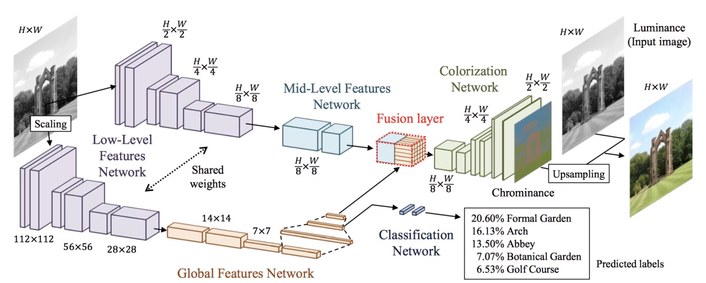 *Satoshi Iizuka, Edgar Simo-Serra, and Hiroshi Ishikawa architecture (2016)*
Judging from empirical evidence in their papers that both neural networks seems to work pretty well, I decided to give it a try and incorporate something similar to their works.
#Shared models
encoder_input = Input(shape=(256, 256, 1,))
encoder_output = Conv2D(64, (3,3), activation='relu', padding='same', strides=2)(encoder_input)
encoder_output = Conv2D(128, (3,3), activation='relu', padding='same')(encoder_output)
encoder_output = BatchNormalization()(encoder_output)
encoder_output = Conv2D(128, (3,3), activation='relu', padding='same', strides=2)(encoder_output)
encoder_output = Conv2D(256, (3,3), activation='relu', padding='same')(encoder_output)
encoder_output = BatchNormalization()(encoder_output)
encoder_output = Conv2D(256, (3,3), activation='relu', padding='same', strides=2)(encoder_output)
encoder_output_shared = Conv2D(512, (3,3), activation='relu', padding='same')(encoder_output)

#Model A
encoder_output = Conv2D(512, (3,3), activation='relu', padding='same')(encoder_output_shared)
encoder_output = Conv2D(256, (3,3), activation='relu', padding='same')(encoder_output)
#Model B
global_encoder = Conv2D(512, (3,3), activation='relu', padding='same',strides=2)(encoder_output_shared)
global_encoder = Conv2D(512, (3,3), activation='relu', padding='same')(global_encoder)
global_encoder = BatchNormalization()(global_encoder)
global_encoder = Conv2D(512, (3,3), activation='relu', padding='same',strides=2)(global_encoder)
global_encoder = Conv2D(512, (3,3), activation='relu', padding='same')(global_encoder)
global_encoder = BatchNormalization()(global_encoder)
global_encoder = Flatten()(global_encoder)
global_encoder = Dense(1024, activation='relu')(global_encoder)
global_encoder = Dense(512, activation='relu')(global_encoder)
global_encoder = Dense(256, activation='relu')(global_encoder)
global_encoder = RepeatVector(32 * 32)(global_encoder)
global_encoder = Reshape([32,32,256])(global_encoder)
#Fusion
fusion_output = concatenate([encoder_output, global_encoder], axis=3)
fusion_output = Conv2D(256, (1, 1), activation='relu', padding='same')(fusion_output)
#Decoder
decoder_output = Conv2D(128, (3,3), activation='relu', padding='same')(fusion_output)
decoder_output = UpSampling2D((2, 2))(decoder_output)
decoder_output = Conv2D(64, (3,3), activation='relu', padding='same')(decoder_output)
decoder_output = UpSampling2D((2, 2))(decoder_output)
decoder_output = Conv2D(32, (3,3), activation='relu', padding='same')(decoder_output)
decoder_output = Conv2D(16, (3,3), activation='relu', padding='same')(decoder_output)
decoder_output = Conv2D(2, (3, 3), activation='tanh', padding='same')(decoder_output)
decoder_output = UpSampling2D((2, 2))(decoder_output)

model = Model(inputs=encoder_input, outputs=decoder_output)
# Finish model
model.compile(optimizer='adam',loss=ssim_loss ,metrics=['mse','mean_absolute_error'])
Included in this model, I have used Relu activation function for the hidden layers and tanh for the last layer. The use of the tanh is because the output layer which are the ab channels have normalized range between -1 and 1, which coincide with the output of tanh. As for the loss function, I decided to use multi-scale SSIM because the results from my previous trial experiments proved that brown is the most closest color to every other color in the spectrum. The image output at the end using MSE as my loss function would be largely just colored in brown. On the other hand, MS-SSIM can help measure the the picture’s similarity as a whole between channels from the target and the generated output. In the above structure, I used a common shared model to encode the input image. The shape gets halved everytime I use a convolutional layer with stride 2. In this case, batch normalization is spreaded out as following Federico (2017). Halfway through convoluting the image into more abstract features, I will halt the convolution in one path, and proceed to form a dense and fully connected layer for the other (which is named global encoder). In the end, I concatenate both paths back again into a fusion output, which is then passed through upsampling layers to return my original image shape.
The benefits of having both globally encoded features and one that stopped at halfway is that the resulting outpt vector contains both defining features of the image and also the overall quality of the picture. This would help in producing a more realistic image when the output is finally produced at the end of the decoding process.
 *SSIM on grayscale; MS-SSIM on 3 channel images*
Pivot to other topic? Or to push on and try other methods?
Unfortunately, after training the above model on 500 epochs, the output did not turn out well with colors like green or blue overtaking the whole picture. In retrospect, even with Colored-Multiscale SSIM, the output turned out to be more grainy than usual. However, this gave me a reason to pursue other forms of models for my coloring problem and thus I encountered DcGANs.
Deep Convolutional Generative Adversarial Network (DcGAN)
 *Deep Convolutional Generative Adversarial Networks*
GANs have been the latest trend in deep learning, where instead of 1 model trying to produce the best fit prediction, we instead have 2 models working in adversarial terms trying to fine tune each other. Akin to the analogy of police and thieves; The generator, which is the thief, will try to generate images as close to the ground truth as possible. On the other hand the discriminator, with the role of the police, will try to differentiate between the ground truth and the generated ouput from the generator. This adversarial relationship forces both models to get better over time, and will help to improve color accuracy of the picture that is generated from the generator.
With the incorporation of both convolutional layers and GANs, we get DcGANs, which utilises convolutional stride in downsampling the input and transposed convolution for upsampling. This makes DcGANs much simpler model that reduces the complexity of the generator and discriminator without causing bottleneck in image quality.
I was amazed with the performance of DcGANs and GANs within the last few years, where a lot of academic papers on computer vision were written. Two versions of a similar DcGANs (aka Pix2Pix) were available for use in in my case. The original was created by Phillip Isola, but was written with PyTorch, and the latter by afflinelayer, written with Tensorflow. I chose to emulate the latter because of the tensorflow compatibility.
In addition, because of the unavoidable problem of long training time for deep learning models, I had to inevitably cut down my sample size from 9.2k images to 2.2k images and also to only use images under the category of people. Hopefully, I would still be able to reach my goal of submission of my capstone before graduation from the course. This is in hope that the model would learn to perform better, especially at predicting colors of grayscale peoeple images.
After looking at the literature for neural architectures, I’ve picked U-net as the neural network that I will aim towards building. This could be said to be a large improvement to the shared model CNN from previous experiments I have tried out. U-net builds on the same concept of concatenating vectors from different levels of convolution as similar to my above example from using different models and concatenating their different outputs. It implements skips between convolution and transpose convolution and only concatenating vectors of same shape. This symmetry is somewhat appealing (aesthetically), but also helps improve image output in detecting anomalies and lessen the load on computational power.
With regards to image preprocessing after switching from CNN to DcGANs, I had to abandon several of the image augmentation using scikit image library, as during tensorflow implementation of the model, I inevitably chose to turn everything into a tensor (as akin to a numpy array). Skimage would not recognise the image datatype for manipulation. However, that is not to say that all hopes for preprocessing the image is lost. Tensorflow does have their own dedicated library for image augmentation under tf.image. Making rotations using tf.image.random_flip_up_down and adjusting contrast, hue and saturation were also available as methods for tensor data types. Also, I decided not to complicate the problem of turning the image into a different color space as the range of outputs and color spaces are too difficult to keep track after all the image augmentations.
New loss terms
With this change in type of model, my loss terms are also now different for each model for the generator and discriminator. For the discriminator, the loss term would be binary crossentropy. This is because the input in the discriminator uses both the ground truth image and the output from the generator. The total loss term for my discriminator is thus created by adding two different crossentropy loss terms; One loss term comes from comparing a tensor of all 1s with the ground truth image, and the other comes from comparing a tensor of all 0s with the generator’s output. This way, the discriminator learns to differentiate between the ground truth better as compared to the generated output.
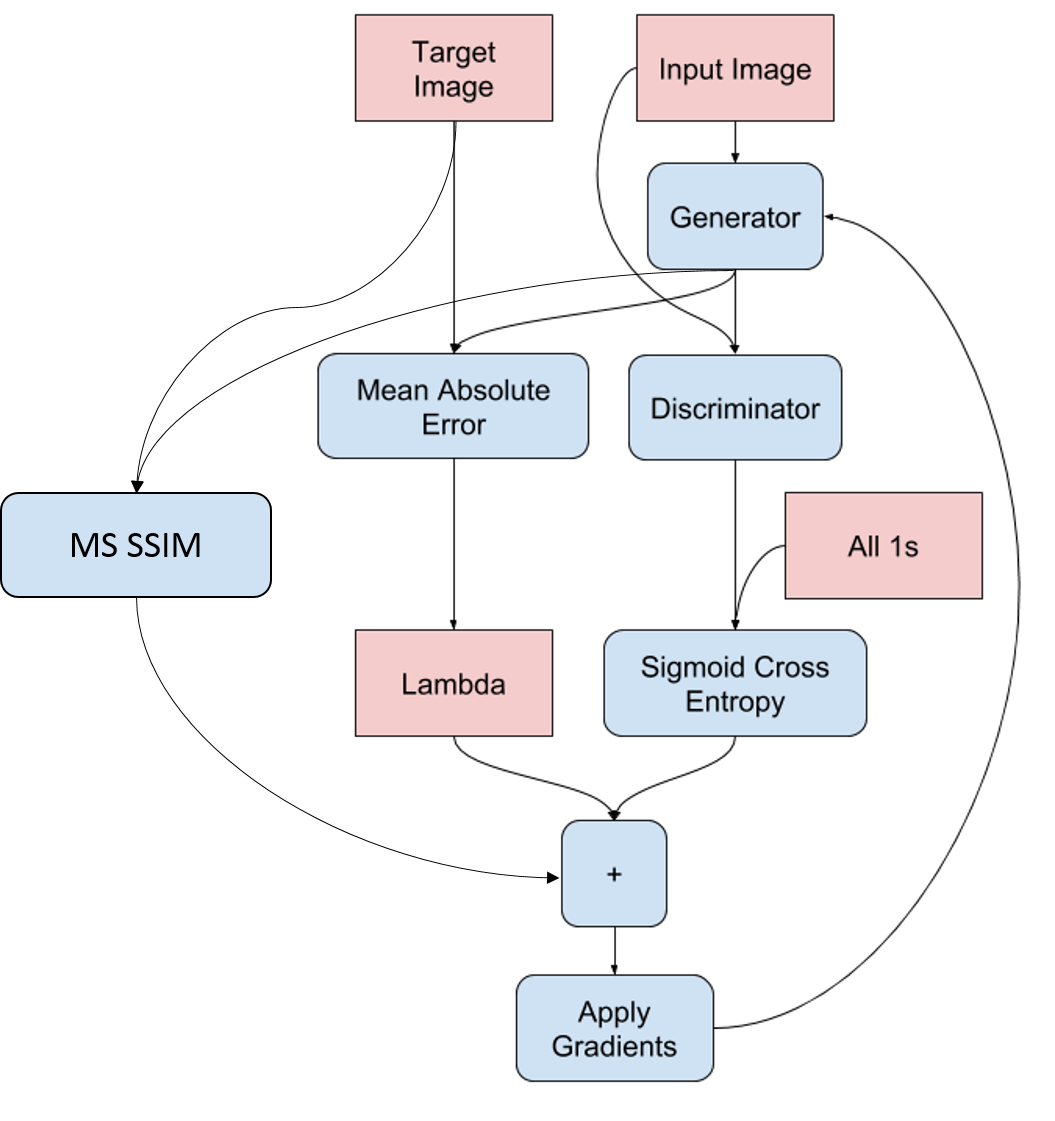 *Generator training diagram*
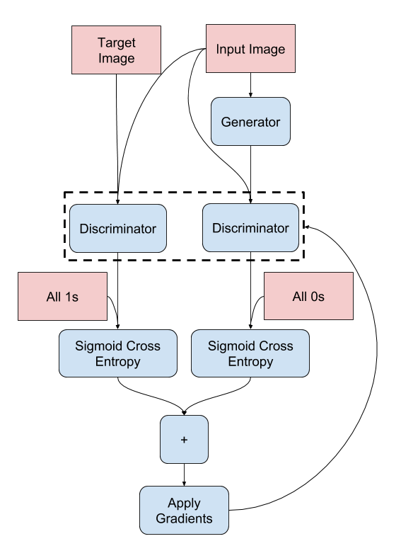 *Discriminator training diagram*
The generator’s loss term on the other hand is the addition of 3 different individual calculations. Firstly, it will utilize the same binary crossentropy of its generated output with all 1s (so as to learn to trick the discriminator). Secondly, an additional loss term of MSE between the ground truth and the generated output and a lambda multiplier of 100 is added to further regularize the generator. Lastly, incorporating MS-SSIM as previously mentioned above, by comparing the similarity score between the output and the ground truth. For the MS-SSIM loss term, because it measures similarity, and the higher the score (range 0 to 1), the closer the comparison; To effectively add this as a loss term, I took the tf.reduced_mean over the 3 RGB layers and transform it by take 1 - the MS-SSIM score.
Finally, at the end, to train the model, I also used the Adam optimizer and these loss terms are respectively applied to their own model (generator and discriminator). Quoted below is the full code that I ran on google Colab with GPU.
# Convu filter to downsample image
def downsample(filters, size, apply_batchnorm=True):
    initializer = tf.random_normal_initializer(0., 0.02)

    result = tf.keras.Sequential()
    result.add(
            tf.keras.layers.Conv2D(filters, size, strides=2, padding='same',
                             kernel_initializer=initializer, use_bias=False))

    if apply_batchnorm:
        result.add(tf.keras.layers.BatchNormalization())

    result.add(tf.keras.layers.LeakyReLU())

    return result

# Convu filter to upsample image
def upsample(filters, size, apply_dropout=False):
    initializer = tf.random_normal_initializer(0., 0.02)

    result = tf.keras.Sequential()
    result.add(
        tf.keras.layers.Conv2DTranspose(filters, size, strides=2,
                                    padding='same',
                                    kernel_initializer=initializer,
                                    use_bias=False))

    result.add(tf.keras.layers.BatchNormalization())

    if apply_dropout:
        result.add(tf.keras.layers.Dropout(0.5))

    result.add(tf.keras.layers.ReLU())

    return result

# Create the generator
def Generator():
    down_stack = [
        downsample(64, 4, apply_batchnorm=False), # (bs, 128, 128, 64)
        downsample(128, 4), # (bs, 64, 64, 128)
        downsample(256, 4), # (bs, 32, 32, 256)
        downsample(512, 4), # (bs, 16, 16, 512)
        downsample(512, 4), # (bs, 8, 8, 512)
        downsample(512, 4), # (bs, 4, 4, 512)
        downsample(512, 4), # (bs, 2, 2, 512)
        downsample(512, 4), # (bs, 1, 1, 512)
          ]

    up_stack = [
        upsample(512, 4, apply_dropout=True), # (bs, 2, 2, 1024)
        upsample(512, 4, apply_dropout=True), # (bs, 4, 4, 1024)
        upsample(512, 4, apply_dropout=True), # (bs, 8, 8, 1024)
        upsample(512, 4), # (bs, 16, 16, 1024)
        upsample(256, 4), # (bs, 32, 32, 512)
        upsample(128, 4), # (bs, 64, 64, 256)
        upsample(64, 4), # (bs, 128, 128, 128)
          ]

    initializer = tf.random_normal_initializer(0., 0.02)
    last = tf.keras.layers.Conv2DTranspose(3, 4,
                                         strides=2,
                                         padding='same',
                                         kernel_initializer=initializer,
                                         activation='tanh') # (bs, 256, 256, 3)

    concat = tf.keras.layers.Concatenate()

    inputs = tf.keras.layers.Input(shape=[None,None,3])
    x = inputs

  # Downsampling through the model
    skips = []
    for down in down_stack:
        x = down(x)
        skips.append(x)

    skips = reversed(skips[:-1])

  # Upsampling and establishing the skip connections
    for up, skip in zip(up_stack, skips):
        x = up(x)
        x = concat([x, skip])

    x = last(x)

    return tf.keras.Model(inputs=inputs, outputs=x)

# Create the discriminator
def Discriminator():
    initializer = tf.random_normal_initializer(0., 0.02)

    inp = tf.keras.layers.Input(shape=[None, None, 3], name='input_image')
    tar = tf.keras.layers.Input(shape=[None, None, 3], name='target_image')

    x = tf.keras.layers.concatenate([inp, tar]) # (bs, 256, 256, channels*2)

    down1 = downsample(64, 4, False)(x) # (bs, 128, 128, 64)
    down2 = downsample(128, 4)(down1) # (bs, 64, 64, 128)
    down3 = downsample(256, 4)(down2) # (bs, 32, 32, 256)

    zero_pad1 = tf.keras.layers.ZeroPadding2D()(down3) # (bs, 34, 34, 256)
    conv = tf.keras.layers.Conv2D(512, 4, strides=1,
                                kernel_initializer=initializer,
                                use_bias=False)(zero_pad1) # (bs, 31, 31, 512)

    batchnorm1 = tf.keras.layers.BatchNormalization()(conv)

    leaky_relu = tf.keras.layers.LeakyReLU()(batchnorm1)

    zero_pad2 = tf.keras.layers.ZeroPadding2D()(leaky_relu) # (bs, 33, 33, 512)

    last = tf.keras.layers.Conv2D(1, 4, strides=1,
                                kernel_initializer=initializer)(zero_pad2) # (bs, 30, 30, 1)

    return tf.keras.Model(inputs=[inp, tar], outputs=last)

# Lambda as defined in the pix2pix journal
lamb = 100
loss_object = tf.keras.losses.BinaryCrossentropy(from_logits=True)

# Discriminator loss terms
def discriminator_loss(disc_real_output, disc_generated_output):
    real_loss = loss_object(tf.ones_like(disc_real_output), disc_real_output)

    generated_loss = loss_object(tf.zeros_like(disc_generated_output), disc_generated_output)

    total_disc_loss = real_loss + generated_loss

    return total_disc_loss

# Generator loss terms
def generator_loss(disc_generated_output, gen_output, target):
    gan_loss = loss_object(tf.ones_like(disc_generated_output), disc_generated_output)

    # mean absolute error
    l1_loss = tf.reduce_mean(tf.abs(target - gen_output))

    #Include SSIM loss
    ssim_loss = 1 - tf.reduce_mean(tf.image.ssim_multiscale(gen_output, target, 1))

    total_gen_loss = gan_loss + (lamb * l1_loss) + ssim_loss

    return total_gen_loss

# Create the optimization to apply gradients to the models
def train_step(input_image, target):
    with tf.GradientTape() as gen_tape, tf.GradientTape() as disc_tape:
        gen_output = generator(input_image, training=True)

        disc_real_output = discriminator([input_image, target], training=True)
        disc_generated_output = discriminator([input_image, gen_output], training=True)

        gen_loss = generator_loss(disc_generated_output, gen_output, target)
        disc_loss = discriminator_loss(disc_real_output, disc_generated_output)

        #Manual loss tracker
        track_g_loss.append(gen_loss)
        track_d_loss.append(disc_loss)

    generator_gradients = gen_tape.gradient(gen_loss, generator.trainable_variables)
    discriminator_gradients = disc_tape.gradient(disc_loss, discriminator.trainable_variables)

    generator_optimizer.apply_gradients(zip(generator_gradients, generator.trainable_variables))
    discriminator_optimizer.apply_gradients(zip(discriminator_gradients,discriminator.trainable_variables))
Results
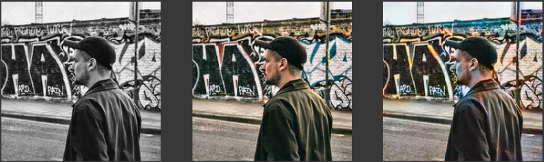
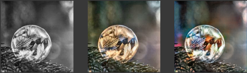
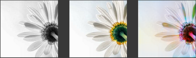
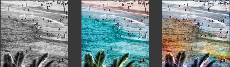
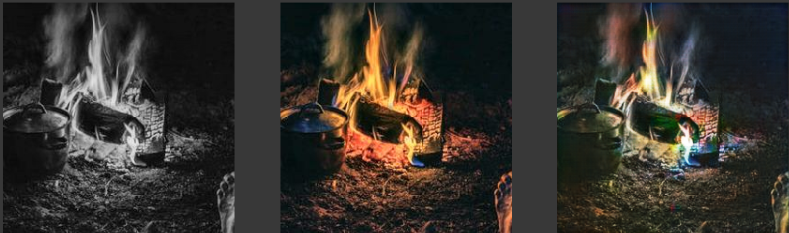
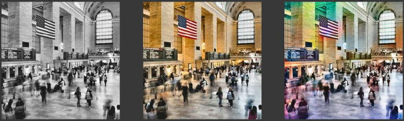
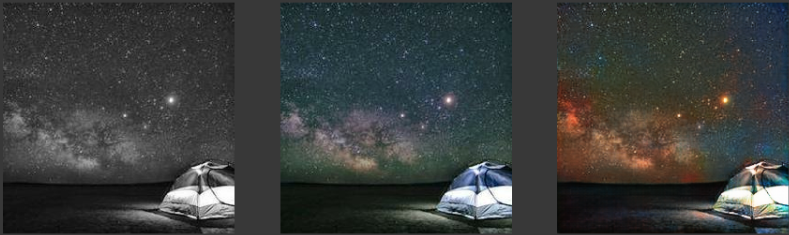
Below are some of the output from the generator. They are in the order of input, ground truth and prediction.

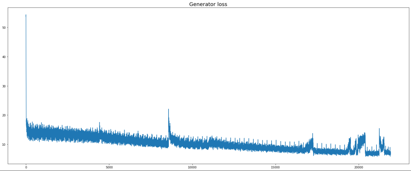
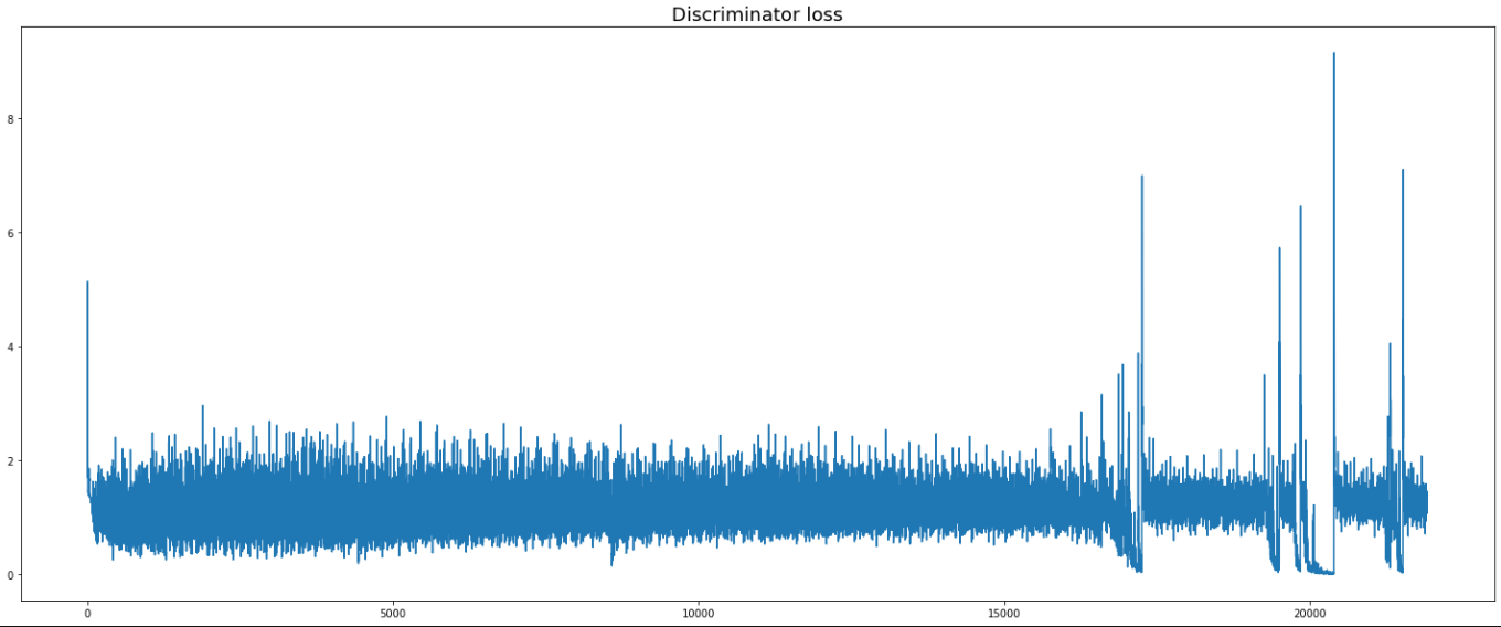
Below is the loss graphs for the generator and discriminator.
Conclusion
In my opinion, there are some mistakes and shortcomings of the DcGAN model as compared to the CNN model. For one, when the image of the person is too large or due to the lack of images that are mainly focused on the person itself, the color of the person tends to blend into the surrounding too. Likely, the defining features for segmenting a person out from the background might not be well captured by the model in DcGANs and thus causing the spillover effect of the colors. Furthermore, included in the dataset were several pictures of people’s silhouettes. These might give the wrong impression to the model about the colors used to represent their skin color, as we also included images of people with different race. The learning might not have been optimized correctly for the generator to understand the play on lighting and brightness in modern day photography. As such, future attempts may look at removing these photos which are photography gimicks that try to stand out from the norm.
My initial problem statement to colorize gray images turned out to be a learning journey in deep learning on my own end. I started out by using CNNs as a simple way to process images that does not use heavy computational power, and I ended up with DcGAN models that had several loss terms that help train the model. Overall, I felt that when I was trying to eliminate the weird colors that kept appearing in my output images, I heavily focused on preprocessing the input and trying to make better loss functions that the generator can learn better. In retrospect, although I did not run a large number of epochs, the loss terms did converge quite early on with few hundred epochs, suggesting that the architecture and process seems to be in the right general direction. Afterall, processing color vision in human only uses that little cone optical nerves as compared to rods which define the optic acuity.
Thank you so much for your time reading my blog post. I hope you had also learnt some lessons with regards to deep learning.